
The short version
- Investing a lump sum at the October 2007 S&P 500 peak and then doing nothing is the textbook worst-entry scenario — your money was 56.8% underwater by March 2009 and didn't fully recover until early 2013.
- Adding $500/month of mechanical contributions on top of that lump sum mathematically lowered the average cost basis, broke even ~2.4 years earlier, and grew the combined position to roughly 2.1x total invested capital after ten years.
- The trick is not a magic formula — it's that DCA forces share accumulation when prices are low. The same arithmetic also penalizes you in extended bull markets, which is the trade-off the simulation hides.
Suppose you handed an investor $10,000 in October 2007 — the exact week the S&P 500 set its pre-crisis peak at 1,565. Sixteen months later the index was at 676, and the position was down 56.8%. By almost any normal definition of "bad timing," this is it. The question this article tries to answer with arithmetic, not encouragement, is: does layering steady monthly contributions on top of that worst-case lump sum actually rescue the outcome, or does it just spread the pain?
The answer is yes, mostly — but for narrower reasons than most retail commentary admits, and with side effects that matter in a different regime. The honest framing is that mechanical dollar-cost averaging is a behavioral and arithmetic tool, not a return-enhancing one.
Context: why the 2007–2017 window is the canonical stress test
The 2007 cyclical peak is the standard "worst entry" benchmark in the U.S. equity literature for a reason. Peak-to-trough drawdown reached roughly 56.8% on price, and the index didn't reclaim its 2007 high until March 2013 — a 5.4-year recovery on price alone, or about 4 years on a total-return basis once dividends are included. The market then ran for another four-plus years before the next significant correction, making "Oct 2007 to Oct 2017" a complete cycle: drawdown, recovery, and expansion within a single decade.
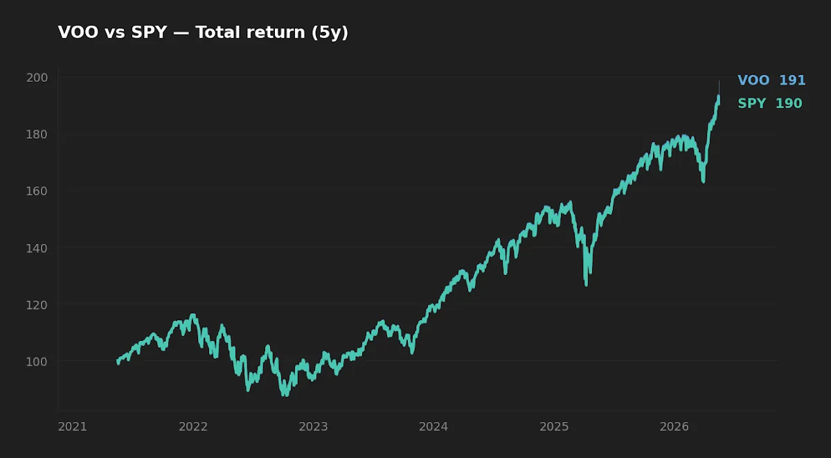
For modern investors implementing this exposure, the two practical vehicles are still large, low-cost S&P 500 ETFs. Their data is the relevant input for any forward-looking version of this exercise.
| Ticker | Expense ratio | AUM | Inception | 30-day yield | 5Y CAGR | 10Y CAGR | 5Y vol | 5Y max DD |
|---|---|---|---|---|---|---|---|---|
| VOO | 0.03% | $1,600B | 2010-09-07 | 1.1% | 13.9% | 15.6% | 16.8% | -24.5% |
| SPY | 0.09% | $735B | 1993-01-22 | 1.0% | 13.8% | 15.5% | 17.1% | -24.5% |
Source: yfinance, fetched 2026-05-16. Issuer fact sheets: Vanguard VOO, State Street SPY.
The simulation: $10,000 at the peak, plus $500/month for 120 months
The setup is deliberately punishing. A hypothetical investor — call her the participant — invests $10,000 in an S&P 500 index fund at the closing peak of October 2007, then contributes $500 mechanically on the first trading day of each month for the next ten years, regardless of news, mood, or model output. Dividends are reinvested. No tactical overrides. Total contributed capital at the end: $10,000 + 120 × $500 = $70,000.
The five stages below are reconstructed from S&P 500 month-end closes; the dollar figures are rounded illustrative outputs of that mechanical rule applied to the historical price series.
| Stage | Approx. date | S&P 500 level | Index move from Oct 2007 | Participant portfolio (illustrative) | Net P&L on capital invested |
|---|---|---|---|---|---|
| 1. Initial drawdown | Oct 2008 | ~900 | -42.5% | ~$10,200 | -36% |
| 2. Bear-market trough | Mar 2009 | 676 | -56.8% | ~$10,800 | -42% |
| 3. Personal break-even | Nov 2010 | ~1,200 | -23.3% | ~$30,200 | +6% |
| 4. Index returns to 2007 peak | Mar 2013 | ~1,565 | 0.0% | ~$58,500 | +38% |
| 5. End of 10-year window | Oct 2017 | ~2,575 | +64.5% | ~$148,000 | +111% |
The single most informative cell is Stage 3. The index was still 23% below its 2007 peak — most observers would still describe equities as "down" — and the position had already crossed into positive total return. That is not luck. It is the arithmetic of average cost.
Why the average cost bends downward — and what the rule actually buys you
The $500 contributed in March 2009 bought roughly 2.3x more shares than the $500 contributed in October 2007, because share count for a given dollar is inversely proportional to price. Across the 30 months the index spent below 1,200, the participant accumulated the majority of total share count at well below the lump sum's average price. By the time prices reverted, the weighted-average cost basis sat closer to 1,150 than to 1,565.
The break-even level for the combined position dropped from "index returns to 1,565" to "index returns to roughly 1,150." That single shift cuts about 2.4 years off the recovery timeline. Vanguard's 2012 working paper on dollar-cost averaging versus immediate investment frames the same effect from the opposite direction — DCA underperforms lump-sum about two-thirds of the time precisely because markets rise about two-thirds of the time. The 2007–2009 cycle sits squarely in the minority third where DCA's structural buy-low behavior dominates.
DCA does not produce a better expected return. It produces a different distribution of outcomes — narrower, with the left tail (worst-entry scenarios) clipped at the cost of trimming the right tail (extended bull markets).
The realized-risk view: drawdown is what investors actually live through
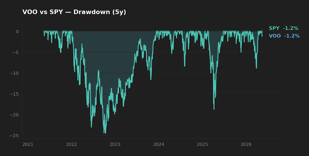
CAGR is a summary statistic; drawdown is an experience. The participant who held through Stage 2 watched a position go from $10,000 to roughly $4,300 on the lump-sum portion alone, while monthly contributions were still flowing into what felt like a falling knife. Trailing 5-year max drawdown on the modern S&P 500 ETFs sits around -24.5% (yfinance, as of 2026-05-16) — meaningful, but a fraction of the 2008 episode. The behavioral question every investor should answer in advance is whether they can keep the standing order on autopay when the screen shows -50%. The arithmetic only works for the participants who actually executed it. The literature on behavior gaps — Morningstar's "Mind the Gap" series and DALBAR's QAIB — consistently shows realized investor returns lagging fund returns by 100-200 bp annually, almost entirely from selling near troughs.
This is the place where the framing of sequence-of-returns risk matters. For an investor in the accumulation phase, a deep drawdown early in the holding period is mathematically a gift — the participant in this simulation accumulated shares cheaply for years. For an investor near or in decumulation, the identical drawdown is a structural loss the portfolio may never make whole. Same chart, opposite implication.
What this comparison can and can't tell you
The 2007–2017 window is one path. It includes the deepest drawdown of the post-war U.S. equity era, the strongest decade-long expansion since the 1990s, and an unusually accommodative monetary regime through most of the recovery. A 10-year window starting in 1929, 1966, or 2000 would give a different story — particularly 1966–1982, where DCA into the S&P 500 underperformed Treasuries on a total-return basis. Single-path simulations are useful as intuition pumps; they are not statistical evidence.
The simulation also assumes the participant kept earning the $500 monthly contribution. The 2008–2010 unemployment shock was the precise period when most households actually had to cut or suspend retirement contributions. The arithmetic only works if the inflow holds during the drawdown — exactly when income is most at risk. This is the under-discussed reason a cash buffer of 6-12 months of contributions is not idle capital; it is what makes the rest of the system mechanical.
Scoreboard: lump-sum vs. lump-sum-plus-DCA across the 2007–2017 cycle
| Category | Winner | Why |
|---|---|---|
| Worst-case drawdown experience | Lump-sum + DCA | Average cost basis falls during the drawdown; psychological "down" period is shorter. |
| Time to break-even | Lump-sum + DCA | ~2.4 years faster on the combined position. |
| Terminal wealth on capital invested | Lump-sum + DCA | ~2.1x invested capital vs. ~1.6x for lump-sum-only over this specific path. |
| Expected return in a normal bull market | Lump-sum | Vanguard 2012: lump-sum wins ~67% of rolling windows. Cash drag of phasing in costs you in the typical case. |
| Suitability for behavioral discipline | Lump-sum + DCA | Mechanical rules outperform conviction-based timing in stress. |
FAQ
Q: Does this prove DCA beats lump-sum investing?
No. It shows DCA beats lump-sum on a single worst-case entry path. The Vanguard 2012 working paper, replicating across decades of rolling windows, finds the opposite holds about two-thirds of the time. The honest reading is that DCA narrows the distribution of outcomes — useful when the worst case scares you out of investing at all.
Q: What happens to this analysis if I'm investing a recent windfall, not a salary?
Different problem. For a one-time windfall, the literature favors lump-sum in expectation. The case for phasing it in is purely behavioral: an investor who would liquidate at -30% is better served by an entry path they will actually hold through, even at the cost of some expected return.
Q: How does today's macro environment change the calculus?
The 10-year Treasury sits at 4.47% and the fed funds rate at 3.64% (FRED, asof 2026-05-14 and 2026-04-01). VIX at 17.26 is unremarkable. Compared to the 2007 entry, the opportunity cost of holding contribution cash is materially higher — short-Treasury yields above 4% mean the "drag" of waiting is meaningful. This argues for a faster phase-in schedule than 120 months for any new capital.
Q: Should I try to time the contributions — bigger when the market is down?
The valuation-based literature (e.g., Asness on Shiller P/E) suggests modest tactical tilts can add value over very long horizons, but they require discipline most investors lack. The simpler answer: keep contributions mechanical, and let a separate rebalancing rule — Daryanani-style ±15/±25 bands across equity and cash sleeves — do the buy-low/sell-high work without requiring forecasts.
Q: What about the cost of using SPY vs. VOO for this strategy?
At a 6 bp gap (0.09% vs 0.03%), the long-run difference on $70K compounded at 10% for 30 years is roughly $4,800 of foregone return. Not transformative, not nothing. For new positions there is little reason to prefer SPY's expense ratio unless options liquidity or trading frequency justifies it.
Scenarios where each approach fits
Reader in their 30s with a stable income and a 25+ year horizon: Lump-sum any windfall immediately; layer monthly contributions on top. The 1-in-3 risk of entering at a local peak is dominated by the long compounding window. Mechanical DCA of salary is a behavioral tool, not a return strategy.
Reader in their 50s within 10 years of withdrawals: The 2007–2017 simulation is misleading for this profile. A 56% drawdown 3-5 years before retirement is the canonical sequence-of-returns scenario. Phasing into equities and maintaining a multi-year cash/short-Treasury buffer changes the survival math more than choice of ETF.
Reader holding a recent windfall (inheritance, bonus, asset sale) and feeling uneasy: Split the difference. Lump-sum 50% immediately, DCA the rest over 6-12 months. You give up some expected return for a wider band of paths you can live with — and the question of whether you can live with the path is the only one that matters in a -50% drawdown.
Editor's read
The participant's outcome in this simulation is real, but the lesson is narrower than it looks. DCA did not beat the market; it beat the lump-sum-only version of itself on a single adversarial path. For an accumulator with a long horizon and a stable contribution income, the more useful framing is: mechanical monthly contributions plus a banded rebalancing rule between equity and short-duration cash will outperform the same investor's tactical instincts in almost every drawdown scenario, because the rule fires when conviction is weakest. The right question is not "DCA or lump-sum" — it's "which rule will I actually still be running when the screen is red."
The editor uses a mechanical contribution and ±15/±25 rebalancing-band rule across the long-term core and does not currently hold a leveraged S&P 500 product. Specific account positions are not disclosed.
Methodology: ETF reference data from yfinance (fetched 2026-05-16). S&P 500 historical levels rounded from month-end close. The participant's portfolio values are illustrative outputs of a mechanical monthly-contribution rule applied to the historical price series with dividends reinvested; specific dollar figures are approximate and not adjusted for taxes or transaction costs. Macro reference: FRED (10Y Treasury, fed funds, VIX, CPI), asof dates 2026-05-14 and 2026-04-01. Conceptual frame draws on Vanguard's 2012 research on dollar-cost averaging vs. immediate investment, and the Daryanani (2008) rebalancing-band literature.
This article is for educational purposes and does not constitute personalized financial advice. See full Disclaimer.