
The short version
- Daily-reset leverage produces a return that, over any non-trivial horizon, is not L times the index — it is L times the daily return, compounded, then taxed by variance, financing, and fees.
- Over the past five years, despite a strongly trending Nasdaq, TQQQ realized 27.0% CAGR versus a theoretical 3× decomposition near 38% — a gap roughly equal to one financing-cost leg.
- Whether decay "wins" depends less on direction than on the joint distribution of trend slope and realized variance, evaluated against today's 4.47% 10-Year Treasury yield.
The phrase "volatility decay" gets repeated so often in leveraged-ETF discussions that it has become a thought-terminating cliché — used either to dismiss daily-reset products entirely, or, on the other side, to argue that the decay is an exaggerated bogeyman that disappears in a strong trend. Neither framing survives a careful look at the math. The honest answer is more interesting: the realized return of a daily-reset leveraged ETF is governed by three superimposed taxes — variance, financing, and tracking — and the question is whether the underlying trend pays them.
This article works through that decomposition using current data for TQQQ, SSO, and QLD against their unlevered references VOO and QQQM, and asks under what conditions each one earns its keep.
Why daily reset is not the same as "3× over time"
A 3× daily-reset ETF promises three times the index's daily return, not three times the cumulative return. That distinction is mathematical, not semantic. To hold constant 3× exposure as NAV moves, the fund rebalances each day — buying after up days, selling after down days. The result is a return path whose log-volatility is roughly 3× the index's log-volatility, and whose expected compound return, under standard log-normal assumptions, decomposes as:
rL ≈ L · μ − ½ · L · (L−1) · σ² − financing − fees
Where μ is the underlying drift, σ is the underlying volatility, L is the leverage multiple, "financing" is the cost of borrowing the leveraged sleeve (tied to short-term rates), and "fees" is the expense ratio. The middle term — the variance penalty — is the part most retail explanations call "decay." It is the only term that grows quadratically with leverage. At L=2 the coefficient is 1; at L=3 it is 3. The variance tax triples between 2× and 3×.
The data table: what we are actually comparing
| Ticker | Name | ER | AUM | Inception | Yield | 5Y CAGR | 10Y CAGR | 5Y Vol | 5Y Max DD |
|---|---|---|---|---|---|---|---|---|---|
| TQQQ | ProShares UltraPro QQQ (3× NDX) | 0.82% | $31.3B | 2010-02-09 | 0.5% | 27.0% | 44.9% | 66.6% | −81.7% |
| QLD | ProShares Ultra QQQ (2× NDX) | 0.95% | $12.0B | 2006-06-19 | 0.2% | 24.9% | 35.8% | 44.8% | −63.7% |
| SSO | ProShares Ultra S&P 500 (2× SPX) | 0.87% | $7.3B | 2006-06-19 | 0.7% | 19.6% | 24.2% | 33.7% | −46.7% |
| QQQM | Invesco Nasdaq 100 (1× NDX) | 0.15% | $82.9B | 2020-10-13 | 0.5% | 17.6% | n/a | 22.3% | −35.0% |
| VOO | Vanguard S&P 500 (1× SPX) | 0.03% | $1,600B | 2010-09-07 | 1.1% | 13.9% | 15.6% | 16.8% | −24.5% |
Data: yfinance daily returns through 2026-05-16; expense ratios and AUM from issuer fact sheets (ProShares TQQQ, QLD, SSO, Invesco QQQM, Vanguard VOO).
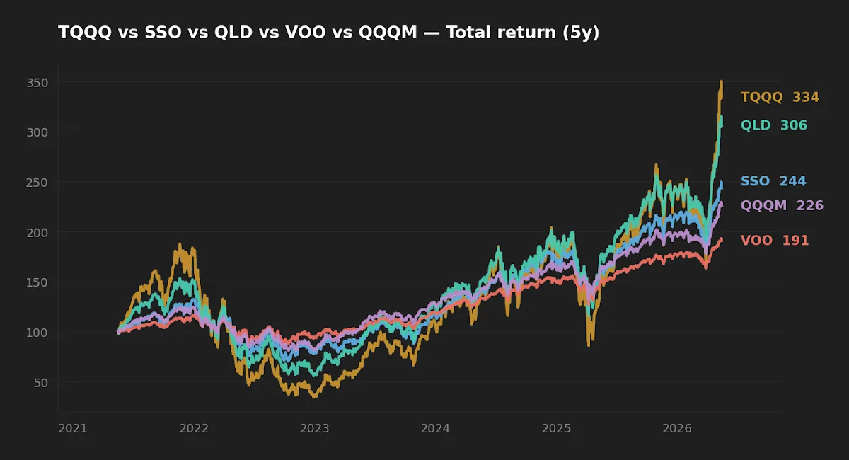
Decomposing the realized 5-year gap
Start with QQQM as the unlevered Nasdaq-100 reference: 17.6% CAGR, 22.3% volatility. The textbook 2× decomposition is:
2 × 17.6% − ½ × 2 × 1 × (0.223)² ≈ 35.2% − 5.0% = 30.2%.
QLD's realized 5Y CAGR is 24.9%. The 5.3-percentage-point gap between the variance-adjusted theoretical and the realized number is essentially the sum of financing cost on the borrowed exposure plus the 0.95% expense ratio — a tight match to what the swap costs and fee schedule would predict in a regime where Fed funds averaged just under 3%.
For TQQQ the same exercise:
3 × 17.6% − ½ × 3 × 2 × (0.223)² ≈ 52.8% − 14.9% = 37.9%.
Realized: 27.0%. Gap: about 11 percentage points annualized. That is the financing leg on roughly 2× NAV of borrowed exposure, plus 0.82% ER, plus a small tracking residual. The pattern is consistent across the 2× and 3× products: the variance term explains decay within a single regime; the financing term explains why "decay" appears worse in high-rate environments.
The math of daily-reset leverage is not a single number but three superimposed taxes — variance, financing, and tracking — and each grows with the leverage multiple in ways most retail explanations conflate.
Why the 10-year picture flatters leverage — and why that is misleading
TQQQ's 10-year CAGR of 44.9% looks heroic. It is also the artifact of a decade in which Fed funds spent most of its time near zero. The financing leg of a 3× swap during 2016–2022 was effectively free; the variance tax during that period was modest because realized volatility, outside of the 2020 and 2022 dislocations, was low. Both ingredients reversed in 2022 and have not fully reverted.
Today's regime, per FRED as of 2026-05-14, sits at a 10Y Treasury yield of 4.47%, Fed funds at 3.64%, VIX at 17.3, and CPI YoY at 3.9%. The implication is direct: every leveraged sleeve held in this regime pays an explicit, non-trivial cost to the swap counterparty before the variance tax is even assessed. A 5-year backtest beginning in 2026 will not look like one beginning in 2016.
For long-horizon readers, the practical conclusion is that the realized 10-year track records of TQQQ, QLD, and SSO are not a forward-looking distribution; they are one regime's worth of evidence, drawn from the most favorable rate environment in modern history. The honest math of daily-reset leverage at a 4% short rate reframes the question more precisely.
Realized risk: drawdown duration matters more than depth
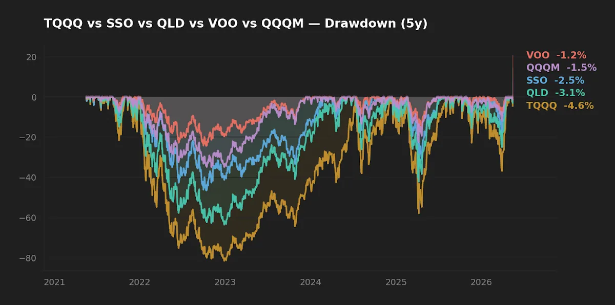
The 5-year max drawdown for TQQQ was −81.7%. The recovery from a drawdown of that magnitude requires a 446% gain to break even. QLD's −63.7% requires a 176% recovery; SSO's −46.7% requires 88%. VOO's −24.5% requires 32%. These are not aesthetic differences. They are the dominant determinant of behavioral failure: most investors who sized leverage on the assumption of "I will hold through anything" did not, in fact, hold through 2022. The drawdown duration — months spent underwater — is what tests conviction, not the print at the bottom.
This is the asymmetry the variance term hides. Variance is a smooth statistic; drawdown is a path-dependent one. Two return series with identical σ can produce very different drawdown experiences depending on the autocorrelation structure of returns. Leveraged ETFs, by construction, amplify negative autocorrelation in choppy markets — the rebalance buys high and sells low at intraday scale.
Scoreboard: who wins on what
| Category | Winner | Why |
|---|---|---|
| Cost (ER + financing) | VOO | 0.03% ER, no financing leg. |
| Realized 5Y return | TQQQ | 27.0% CAGR — but in a strongly trending Nasdaq regime with falling-rate tailwinds for most of the window. |
| Realized 5Y risk-adjusted return | VOO | 13.9% / 16.8% vol ≈ 0.83 raw ratio; TQQQ ≈ 0.41. |
| Drawdown survivability | VOO | −24.5% peak-to-trough is within most investors' behavioral budget; −81.7% is not. |
| Suitability as long-term core | VOO / QQQM | Daily-reset products are not engineered as buy-and-hold cores; they are tactical sleeves. |
FAQ
Does TQQQ mathematically decay to zero? No. The fund cannot go to zero on a single day's move because it resets daily — a 33% drop in the underlying would be required, and the prospectus permits intraday halts. Over multi-year horizons the price can fall by an arbitrarily large fraction in a sufficiently bad regime, but the "decay-to-zero" framing confuses the variance penalty with a structural bankruptcy mechanism.
Why does TQQQ underperform 3× the Nasdaq's cumulative return? Because it never targeted 3× the cumulative return. It targets 3× the daily return. The two are equal only in a single trading day with no rebalance. Over multiple days, the realized result is the cumulative product of daily 3× returns, which under non-zero variance is strictly less than 3× the cumulative product of 1× returns.
Is periodic rebalancing into a leveraged ETF better than buy-and-hold? In simulations using the past decade's data, disciplined band-rebalancing of a small leveraged sleeve against a 1× core has improved risk-adjusted outcomes versus naive buy-and-hold of the leveraged ETF. It does not make the leveraged sleeve a substitute for the core. See why capital preservation governs leveraged outcomes.
How does the current rate environment change the calculus? Materially. With Fed funds at 3.64% (FRED, 2026-04-01), the swap financing leg in a 3× product costs roughly twice the fund's NAV times the short rate annually. That is several percentage points of headwind before any variance term is applied — and it is the largest single difference between today and the 2016–2021 backtest.
Are 2× products structurally safer than 3× for long horizons? The variance term grows from 1× to 3× as the multiple goes from 2× to 3×. The financing leg roughly doubles. The drawdown depth at any given underlying drawdown roughly scales. None of these make 2× "safe" — they make it less unsafe per unit of upside captured. Whether that trade-off is worth taking depends on the holder's behavioral budget, not the math.
What this comparison can and cannot tell you
The 5-year and 10-year windows shown above are single realizations of a path-dependent process. They include one major drawdown (2022) and several smaller dislocations, but they do not include a prolonged sideways regime of the kind that hit Japanese equities for two decades after 1989, or US equities from 1966 to 1982. Volatility-decay arguments are most punishing in exactly those environments — and they are absent from the sample. The published numbers tell you what happened. They do not bound what could.
Scenarios where each instrument might fit
Long-horizon investor, no current leverage, conviction in long-term US equity drift: VOO or QQQM as the core; consider a small (5–15%) tactical sleeve in a 2× product only if rebalancing discipline and behavioral budget are both genuinely tested.
Investor with existing concentrated equity exposure (e.g., employer stock): Adding TQQQ or QLD compounds, rather than diversifies, the existing tail risk. Unlevered international and factor exposure is the asymmetric trade here, not more Nasdaq beta.
Investor with a defined tactical horizon (under 12 months): Daily-reset products were designed for this case. The variance tax over weeks is small; the financing tax over weeks is small; tracking is reasonably tight. The instrument fits its design specification.
Editor's read
Daily-reset leveraged ETFs are honest instruments with a clearly specified design. They are not engineered to be long-term cores, and the realized data — even in the most favorable possible decade — does not argue they should be repurposed as such. Where leverage genuinely earns its place in a long-horizon framework, the editor's preference is to obtain it through portfolio construction (factor tilts, modest cash drag reduction) rather than through products whose variance penalty triples at the 3× step. The math is not the bogeyman. The financing leg, in a 4% rate regime, is.
The editor does not hold TQQQ, QLD, or SSO; the editor holds VOO and QQQM as part of a long-term core allocation.
Methodology
Price and return data: yfinance daily total-return series, pulled 2026-05-16. CAGR and volatility computed on log returns over the 5-year and 10-year windows ending 2026-05-16. Max drawdown computed as peak-to-trough on the cumulative total-return series within the 5-year window. Expense ratio, AUM, dividend yield, and inception sourced from each issuer's most recent public fact sheet. Macro context (10Y, Fed funds, VIX, CPI YoY) from FRED, as-of dates noted inline. Theoretical leverage decomposition uses the standard log-normal approximation rL ≈ Lμ − ½L(L−1)σ²; financing approximation uses (L−1) × short rate.
Key takeaways
- The decay debate misses the structure: variance, financing, and fees are three distinct taxes, not one. Each scales differently with leverage.
- A 5-year CAGR of 27.0% for TQQQ understates the variance/financing drag because the window straddles the lowest-rate decade in modern history.
- At today's 4.47% 10Y and 3.64% Fed funds, the financing leg alone is several percentage points annualized for a 3× product — paid before any market move.
- −81.7% drawdowns test behavior, not math. The largest realized cost of leveraged-ETF investing is forced selling at the bottom.
- Daily-reset products fit tactical windows. They are not designed substitutes for an unlevered long-term core, and the data does not argue otherwise.
This article is for educational purposes and does not constitute personalized financial advice. See full Disclaimer.