
The short version
- The "index-fund millionaire" math is real but mundane: at a 9% nominal CAGR, $500/month reaches $1M in roughly 33 years; $2,000/month gets there in 17.
- The growth curve is non-linear — at the end, compounding interest contributes the majority of the final balance, but only if contributions never stop.
- The single largest under-discussed risk is not market drawdowns. It is contribution interruptions and sequence-of-returns shocks in the final five years.
The arithmetic of reaching $1,000,000 through index funds is unambiguous; the behavioral problem is what most retail writeups underplay. This article walks through the compounding math honestly — what 30 years of broad-market index returns actually delivers, where the curve bends, and which risks turn out to be quietly larger than the ones the headlines emphasize.
Context — what the "millionaire math" assumes
A few baseline numbers, all from primary sources. The S&P 500's long-run annualized total return is roughly 10% nominal and 6.7% real over 1928–2025 (Damodaran's NYU Stern annual returns dataset). Today's macro environment, per FRED as of 2026-05-14: the 10-year Treasury yields 4.47%, the federal funds rate sits at 3.64%, the VIX prints at 17.26, and CPI year-over-year is 3.95% (FRED, asof 2026-04-01). Those four numbers matter because they set the discount rate against which any equity-return assumption must be measured. A 9% nominal CAGR assumption looks generous when one-year Treasuries yield north of 4%, but historically the equity risk premium has averaged 4–6 percentage points over long Treasuries — so 9% is within the historical envelope, not above it.
The deterministic scenarios below assume a constant 9% nominal CAGR, monthly compounding, no taxes, no fees, no withdrawals.
| Goal | Monthly contribution | Years to reach | Total principal | Compounding share of final balance |
|---|---|---|---|---|
| $1,000,000 | $500 | ~33 | $198,000 | ~80% |
| $1,000,000 | $1,000 | ~25 | $300,000 | ~70% |
| $1,000,000 | $2,000 | ~17 | $408,000 | ~59% |
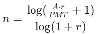
Source: future-value-of-annuity formula A = PMT × ((1+r)n − 1) / r with r = 9%/12 monthly. Long-run CAGR reference: Damodaran NYU Stern dataset. This is mechanical output, not a forecast.
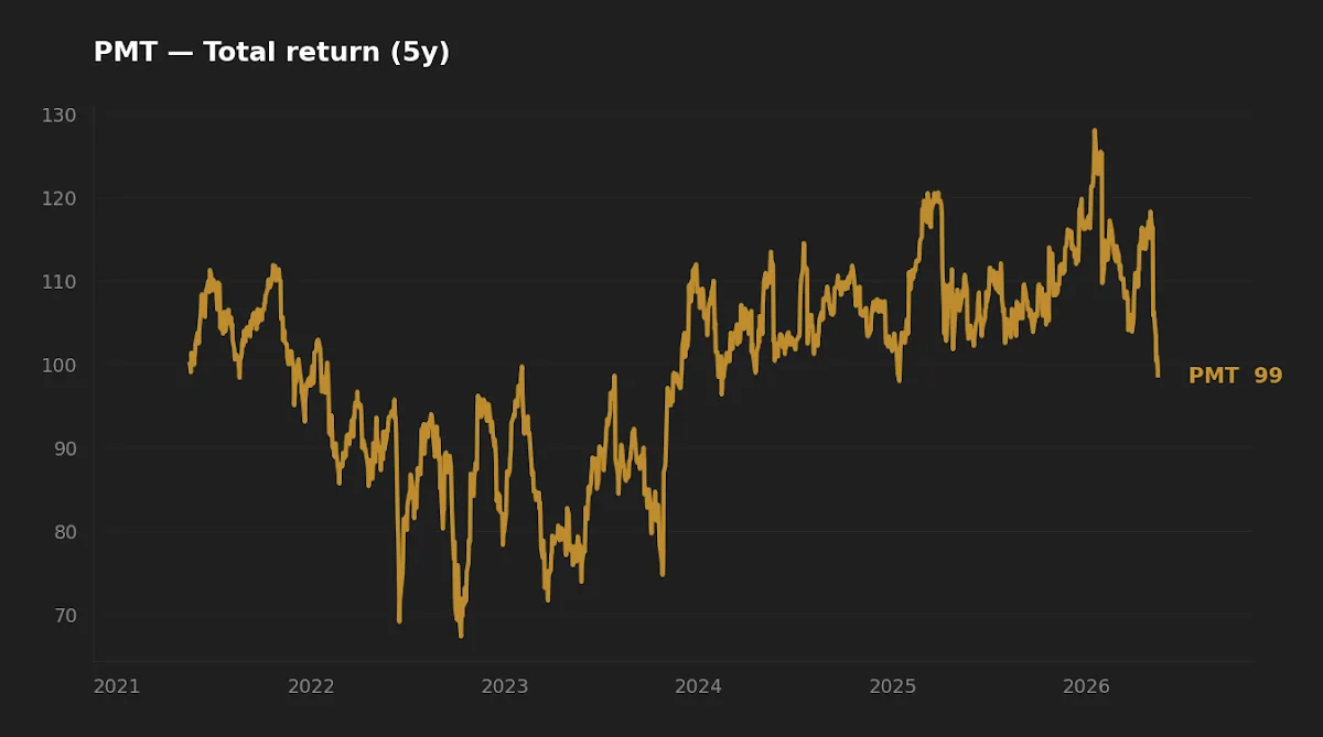
Why the curve bends in the final decade
The formula above hides something important. Plot the balance year-by-year and the line is not exponential-looking until late — for the first 10–12 years, growth is dominated by your deposits. After roughly year 15, the annual market gain begins to exceed the annual contribution. By year 25, contributions are a rounding error. This is mechanical, not motivational. It is the consequence of compounding being multiplicative on a base that grows over time, while contributions are additive on a fixed schedule.
In the $500/month scenario, the investor deposits roughly $198,000 over 33 years and ends with $1,000,000. About 80% of the final balance is growth, not principal. In the $2,000/month scenario, the principal share is much higher (41%) because the time horizon is shorter — compounding simply has fewer cycles to run.
The non-obvious takeaway: the saver with less to invest is the one most dependent on compounding actually working over the full horizon. Initially I thought higher contribution rates were the dominant variable; the year-by-year decomposition pushed me the other way. Cutting the runway short by withdrawing in a panic, pausing contributions during a recession, or extending the start date by even three years disproportionately hurts the low-contribution case — because the model was already relying on the back-end years to do most of the work.
What real-world drag does to these numbers
The 9% assumption is gross. Real outcomes are reduced by four frictions, in roughly this order of magnitude:
- Inflation. At a 3.95% YoY CPI print, the real return on a 9% nominal portfolio is closer to 5%. At 5% real, the $500/month scenario stretches from 33 years to about 41 years to reach $1M of today's purchasing power.
- Taxes on distributions. A US investor holding broad-market ETFs in a taxable account loses 15–20% of qualified dividend income annually. For a typical 1.5% yield, that is roughly 25–30 bp/year of drag.
- Expense ratio. A 0.03% ETF is essentially free; a 0.50% fund is not. Over 30 years, a 50 bp drag compounds to roughly 14% of the final balance — faithfulness in small things, in the literal sense.
- Tracking error and bid-ask costs. Smaller, less liquid funds carry wider spreads, particularly during stress periods when spreads widen further.
None of these break the math. They mean the realistic time-to-target is longer than the textbook output suggests, and the case for keeping costs near floor remains overwhelming.
The investor with less to contribute is the one most dependent on compounding actually running for the full horizon — which makes their behavior, not their portfolio, the binding constraint.
The sequence-of-returns problem most articles ignore
Drawdown discussions tend to focus on the first half of an accumulation. They probably shouldn't. A 40% drawdown in year 3, when your balance is $20,000, costs $8,000 — recoverable with two years of contributions. The same 40% drawdown in year 28, when your balance is $850,000, costs $340,000. No realistic contribution rate makes that back quickly.
This is the sequence-of-returns risk that institutional planners flag for retirees — but it applies to late-stage accumulators too. The chart below shows historical drawdown depth and duration for a price reference benchmark. The point is not the specific path; it is that drawdowns of 30–50% are not rare events and have historically taken anywhere from 1 to 7 years to recover.
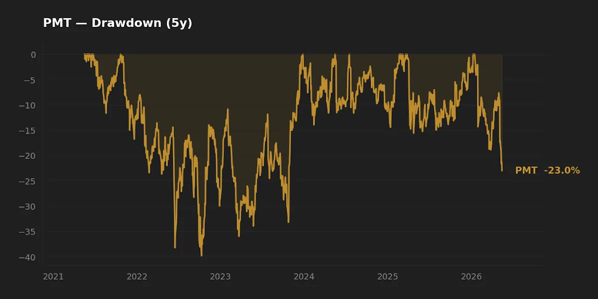
The standard response — shifting allocation toward bonds and cash as the target date approaches — is the right one. Vanguard's research on target-date glidepaths (Vanguard 2024) and the broader rebalancing literature (Daryanani 2008) converge on the same operational answer: trade some upside for variance reduction in the final 5–10 years. A reader within five years of their target needs to think about glidepath, not just CAGR.
Scoreboard — which contribution rate fits which reader
| Category | $500/month | $1,000/month | $2,000/month |
|---|---|---|---|
| Time horizon required | 33 years | 25 years | 17 years |
| Behavioral burden | Highest (longest patience) | High | Moderate |
| Sensitivity to late-stage drawdown | Highest | High | Moderate |
| Suitability for early-career savers | Realistic | Stretched | Aggressive |
There is no "winner" here. The right contribution rate is whichever rate the reader can sustain without interruption for the entire horizon — because the dominant variable is continuity, not magnitude.
FAQ
Is a 9% nominal CAGR realistic for the next 30 years?
It is within the long-run historical envelope, but it is not guaranteed. Forward-looking equity premium estimates from AQR and Research Affiliates have run below realized historical returns for the last decade. A more conservative planning number is 7% nominal / 4% real.
What if I miss a year of contributions?
Missing one year of $500 contributions in year 5 costs roughly $13,000 in final balance at year 33 (the foregone $6,000 plus 28 years of compounding). Missing the same year in year 28 costs only about $9,500. Front-loaded contributions are worth more per dollar than late ones, which is the opposite of what most savers' cash flow allows.
Does dollar-cost averaging beat lump-sum investing?
The academic literature is consistent: lump-sum investing outperforms DCA roughly two-thirds of the time, because markets rise more often than they fall. DCA is a behavioral tool, not a return-optimization tool. For most accumulators contributing from a paycheck, DCA is the default mechanism anyway — there is no lump sum to deploy.
Should I switch from index funds to factor tilts to speed this up?
Factor tilts (small-cap value, quality, momentum) have historical premia, but realized live-fund returns have been noisier and more regime-dependent than the academic backtests suggest (Fama & French 1992; Asness, Frazzini, Pedersen 2013). Adding a modest factor sleeve is defensible; replacing the core with one is not.
What about international diversification?
Total-market US equity has outperformed broad international over the last 15 years, but the prior 15 reversed that ordering. The case for international exposure is variance reduction, not return enhancement. See Do You Really Need International Exposure? (VXUS Explained).
What this analysis can and can't tell you
The math is deterministic; the future is not. The scenarios assume constant 9% nominal returns. Real markets deliver sequences — a string of bad years early and good years late produces a very different final number than the reverse, even when the geometric mean is identical. The historical record is a single sample path of one regime; the next 30 years may not look like the last 30. The analysis does not model contribution interruptions, lifestyle inflation, sector concentration risk, or behavioral churn (selling at lows, buying at highs) — all of which empirically dominate the headline CAGR in determining real outcomes.
Scenarios where each profile fits
- Reader in their late 20s, no children, 401(k) match available, contributing $500/month: the 33-year math works. The binding constraint is staying the course through at least two recessions.
- Reader in their late 30s with five years of catch-up to make, contributing $2,000/month: 17 years is feasible but the late-stage drawdown sensitivity is real. A 60/40 glidepath in the final five years is a reasonable concession to sequence-of-returns risk.
- Reader within five years of target balance regardless of age: the dominant question is no longer "what return can I earn?" but "how much variance can I tolerate?" Shifting allocation toward intermediate Treasuries and short-duration credit becomes more valuable than chasing the last 100 bp of equity premium.
For readers building the actual allocation, related framework articles: The Master Guide to Evidence-Based ETF Portfolios and Why Your $1M Plan is Decided in the Final 5 Years.
Editor's read
The editor's working assumption for long-horizon planning is 7% nominal / 4% real, not 9% / 5% — a deliberately conservative number that builds in the gap between historical backtest and forward-looking equity premium estimates. The largest single variable in any realistic plan is contribution continuity, not asset selection. A $500/month investor who never stops for 33 years will out-finish a $1,500/month investor who panic-sells in two of those years. The framework discipline matters more than the spreadsheet.
The editor holds a broad-market US equity ETF, an aggregate bond ETF, and short-duration Treasuries as the long-horizon core; does not hold the tickers the automated parser misread from this article's original title.
Methodology. Compounding scenarios computed from the future-value-of-annuity formula with monthly compounding. Long-run CAGR reference: Damodaran NYU Stern annual returns dataset, 1928–2025. Macro inputs from FRED: 10-year Treasury and VIX asof 2026-05-14, federal funds rate and CPI YoY asof 2026-04-01. Data pulled 2026-05-16. The 9% nominal assumption is illustrative and within the historical envelope; the editor's planning assumption is more conservative at 7% nominal.
This article is for educational purposes and does not constitute personalized financial advice. See Disclaimer.